A short history of the beginning of Quantum Mechanics (1853 – 1926) ……
- Consider the visible emission spectrum of hydrogen – the 4 most prominent visible lines start the Balmer series of lines (H-alpha, H-beta, H-gamma, H-delta). This was the state of affairs in the mid-19th century following the first observations of the spectrum of hydrogen by Angstrom (in 1853). Angstrom’s first observations of line emission was by observing the spectrum of an electrical spark in a gap that was in an environment of atmospheric pressure hydrogen gas. He later improved these measurements by observing the spectrum in a rarified hydrogen environment in a low-pressure gas discharge tube. Angstrom also made careful measurements of Fraunhofer lines in the spectra of stars. Fraunhofer (in 1814) was the first to observe dark absorption lines in the spectrum of the sun.
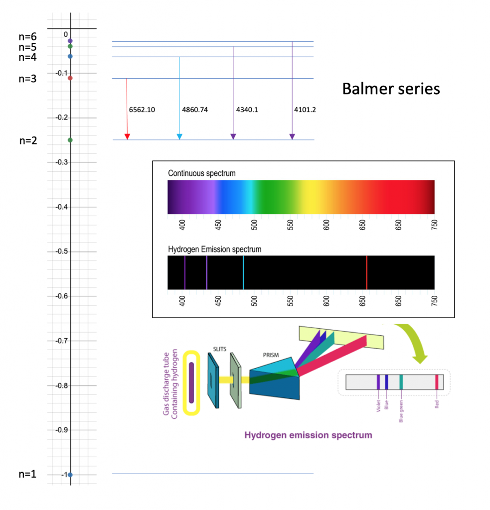
(Figure above includes components from: https://www.thoughtco.com/definition-of-balmer-series-604381 and https://byjus.com/chemistry/hydrogen-spectrum/)
2. Balmer (in 1885) figured out a formula that predicted the wavelengths of the first 4 lines of the visible spectrum for hydrogen. His formula for these first 4 lines was: lambda = 3645.6 * m^2 / (m^2 – 2^2) where lambda is the wavelength in units of 10^-10 meters (now known as Angstroms), and m was an integer series starting with m=3 – he used this same formula to match the wavelengths of 10 additional ultraviolet lines in the series, extending the series up to m=16. The ultraviolet lines came from observations of the spectra of stars. This series of wavelengths is now known as the Balmer series.
3. Rydberg (in 1890) expanded on Balmer’s formula for use with other atoms (especially alkali atoms) – Rydberg’s version of the formula is inverted and expressed as a measure of reciprocal wavelength: (1/lambda) = 109721.6 * (1 / n^2 – 1/m^2). This is the form that is used today. The current value of the constant in this formula (now known as the Rydberg constant) is 109737.316 in units of cm^-1 (also known as reciprocal centimeters or wavenumber). Balmer and Rydberg’s work inspired Nils Bohr to develop a theory that would explain these formulas.
4. Planck (in 1900) introduced a theory to explain the continuous spectral emissions of a hot body (blackbody spectrum). Planck’s theory introduced the concept of quantum states of energy E = h * nu, where E is energy, nu is frequency, and the constant h. h is now known as Planck’s constant.
5. Bohr (in 1913) introduced a theory of the atom now known as the “old quantum theory” that combined classical ideas with the then new quantum ideas of Planck. Bohr postulated that an atom was akin to a planetary system with electrons orbiting in circular orbits. Bohr’s model introduced the concept of stationary states and a lowest state with quantum number n=1. Higher energy states (circular electron orbits) had increasing quantum numbers n=2,3,4, …. Bohr’s work followed the work of Rutherford (in 1911) who postulated that an atom was made of a positive charge center surrounded by electrons. Bohr was able to derive the Rydberg formula, as well as an expression for the Rydberg constant based on fundamental constants of the mass of the electron, charge of the electron, Planck’s constant, and the permittivity of free space.
6. Sommerfeld (in 1916) expanded on Bohr’s ideas by introducing elliptical orbits into Bohr’s model. Sommerfeld’s improvement allowed the Bohr model to explain the splitting of the Balmer lines when the hydrogen atom was in an electric field. Electric field splitting of lines is known as the Stark effect. Today the “old quantum theory” is known as the Bohr-Sommerfeld Model.
7. de Broglie (in 1924) in his PhD thesis developed the idea of matter waves that have a wavelength given by lambda = h / p, where h is Planck’s constant and p is the particle momentum.
8. Schrodinger (in 1926) developed a theory that launched the field of Quantum Mechanics, known as Schrodinger’s equation. It is a non-relativistic theory that is used today to describe atomic structure.
——————————————————————————-
A detailed timeline with links to the original papers follows ….
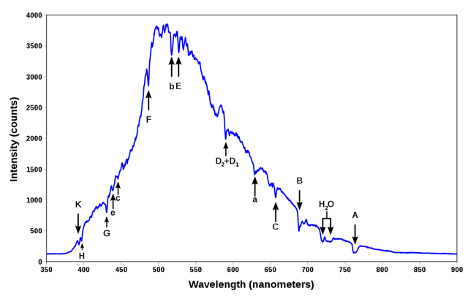
1814 – Fraunhofer observes dark lines in solar spectrum – gives major lines a letter based designation – the C line is H-alpha, the F line is H-beta, the G’ line is H-gamma, and the h line is H-delta. D1/D2 are the doublet lines of Sodium.
Fraunhofer 1814 Denkschriften der Königlichen Akademie der Wissenschaften zu München
1853 – Angstrom first to observe visible spectrum of hydrogen – atmospheric pressure/electric spark/Leyden Jar
1868 – Angstrom’s detailed map of the solar spectrum
1870 – Virial Theorem by Classius – applies for all stable systems: for 1/r2 force law with particles in stable orbit: <T> = – 0.5 <V>
1885 – Balmer formula matching wavelengths Angstrom’s hydrogen measurements of 4 spectral lines – uses formula to analyze spectral observations from stars – formula matches the wavelengths of ten additional hydrogen spectral lines
MGL translation of Balmer paper
1890 – Rydberg formula for spectral lines in alkali atoms
1897 – Zeeman shows that magnetic field splits spectral lines
Zeeman Philosophical Magazine 1897
1897 – Larmor theory of magnetic field effect on spectra, and Radiation from moving charges
1900 – Planck theory of blackbody radiation: E = h * nu
Planck (1900), Distribution Law
1911 – Rutherford model of atom – nucleus plus orbiting electrons
1913 – Bohr model of atom – circular orbits – derives Balmer formula, Rydberg constant, radius of atom, and more
Bohr1920_Article_ÜberDieSerienspektraDerElement
1914 – Stark shows Balmer lines split in an electric field
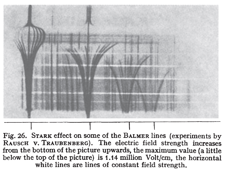
(Figure above from Bethe and Salpeter’s 1957 book on Quantum Mechanics of one and two electron atoms)
1915 – Sommerfeld’s improvement to Bohr model – elliptical orbits – angular momentum added to the Bohr model
1924 – deBroglie hypothesis – PhD thesis under Langevin – matter waves: lambda = h / p
1925 – Goudsmit and Uhlenbeck – introduce the concept of electron spin – electrons are magnetic!
1926 – Schrodinger atomic model
——————————————————————————-
Now let’s use the Bohr model to derive some important relationships for atomic hydrogen ……
- We will use the following concepts ….
- Kinetic energy = T = 0.5 * m * v^2; m is the mass of the electron
- Potential energy = V = – e^2 /((4*pi*epsilon0)*r); epsilon0 is the permittivity of free space
- <T> = -0.5*<V>; Virial Theorem – applied to stable orbits and 1/r^2 force law
- Momentum = p = m * v
- Lambda = h / p; deBroglie wavelength hypothesis; h is Planck’s constant
- Total energy = W = T + V
- Delta energy = h * nu; Planck hypothesis – where nu is the frequency of the photon that is emitted when a large orbit decays (that is, it loses energy) to a smaller orbit; h is Planck’s constant
- Assume that the proton is infinitely massive
- Consider only circular orbits
- Assume that the stationary orbits have integral number of deBroglie wavelengths
- Ground state (n=1) has 1 deBroglie wavelength
- First excited state (n=2) as 2 deBroglie wavelengths, and so on
- From these ideas we will be able to get expressions for several important quantities ….
- Bohr radius = a0 = this is radius of the ground state (n=1) – which matches the most probable value of the radius as predicted by solution to Schrodinger’s Equation
- Radius of orbits for all of the excited states -> which is n^2 * a0; also matches Schrodinger’s predictions
- The energy of the atom (W) as a function of the quantum number n -> which scales as -1/n^2
- A value for the Rydberg constant is derived based on fundamental constants of e, m, epsilon0
- The Rydberg formula is understood by combining the Planck hypothesis and the value determined of the energy (W) of the atom in various orbits
- Velocity of the electron in orbits for all states -> the velocity scales as 1/n; the velocity in the ground state is alpha * c; where alpha is the fine structure constant (approx 1/137) and c is the speed of light
- Orbital period of the orbit which matches 1/frequency of the photon emitted when the atom decays from a high orbit to the next lower orbit -> that is when orbit for state n decays to state n-1; this applies in the limit of large n, known as the correspondence limit
- Bohr magneton = u0; an expression is determined based on fundamental constants for this important property of the hydrogen atom; u0 * B, where B is energy shift in a magnetic field matches one aspect of the observed splitting of spectra by a magnetic field -> Zeeman effect; Zeeman effect is not fully described until one adds in the extra effect of electron spin (electron magnetism) that was discovered by Goudsmit and Uhlenbeck in 1924.
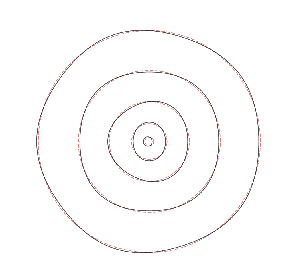
Below is an illustration of the Bohr atom for the lowest 5 orbits (n=1,2,3,4,5) – the circular orbits are shown in red dashed circles – notice that the lowest state, which has radius a0, has a circumference that equals one deBroglie wavelength, that is deBroglie wavelength for n=1 is 2*pi*a0 – the second state has a radius that is 2^2 * a0 = 4 * a0 – its circumference corresponds to two deBroglie wavelengths, that is deBroglie wavelength for n=2 is 2*pi*4*a0, and so on – derivations to follow ….
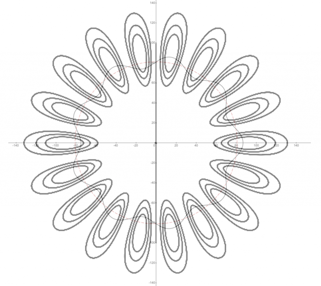
When compared with the Schrodinger Equation solution, the Bohr model is off by 1 deBroglie wavelength – that is, it overestimates the number of deBroglie wavelengths by 1 for each level. So according to Schrodinger’s analysis for n = 1, the number of deBroglie wavelengths is 0, n = 2 the number is 1, and so on. We can see this by comparing an overlay of the Schrodinger solution (contour lines indicate probability of electron position – probability is proportional to the square of the wavefunction – wavefunction goes positive and then negative – the square is positive definite – so there are two lobes for each deBroglie wavelength) for n = 10, with the Bohr solution (red dotted circle with wavy black line indicating deBroglie wave) for n = 9 – in these two cases there are 9 deBroglie wavelengths – the units in the graph below is in ao (that is, the Bohr radius) – so you can see that the Schrodinger solution for n = 10 has a radius of about 100 * a0, and the overlay from the Bohr model for n=9 has a radius of precisely 81 * a0. When the quantum number increases, the relative radius error between Schrodinger and Bohr decreases. To recap, the Bohr model does a reasonable job at estimating the size of the atom, but misses the number of deBroglie waves in an orbit by 1.