Project Goal
This project aims to model the Hydrogen atom using two primary physical mechanisms: the Coulomb force to represent the electrostatic potential between the proton and electron, and Larmor radiation to account for energy loss due to electromagnetic radiation. By constructing this simulation, I hope to compare the results to those of previous contributors who used different software platforms for similar analyses.
Getting Started: The Two-Body Problem
To build foundational understanding, I began by modeling the classic two-body problem. Rather than jumping directly into the hydrogen atom, I chose to first simulate a gravitational system involving two general masses. This served as a conceptual stepping stone and helped me get familiar with COMSOL’s capabilities.
While researching, I came across an online example simulating a satellite orbiting Earth—complete with an mph file. This example, created by Walter Frei (a well-known contributor to COMSOL’s learning resources), became a valuable reference for me. It was also my first experience working with the Global ODEs and DAEs interface in COMSOL.
Tutorial Resource:
Walter Frei’s COMSOL tutorial – a helpful guide for beginners and advanced users alike.
(You can download the model from the bottom of his webpage.)
As a test of my understanding, I created a simple orbital simulation: a randomly shaped object orbiting Earth at a radius roughly equivalent to the Moon’s distance. The force governing the motion was gravitational, and the model was built using with the Global ODEs and DAEs physics. This exercise helped me get familiar with setting up the mechanical equations, defining initial conditions, and choosing appropriate solver configurations. It served as an early confidence to building step before transitioning to the more complex task of modeling atomic-scale systems.
This write up was created to test my knowledge and confirm I knew the parts to the COMSOL
These were 2 orbits that I created
From Orbital Mechanics to Atomic Modeling
After refining the initial setup, I began modifying the conditions to more closely reflect a true two-body system. These adjustments included simplifying the model to remove unnecessary complexities, such as matrix definitions used in satellite-orbit problems. Unlike Walter Frei’s satellite model—which required transformation into the satellite’s reference frame—this version remains entirely in an inertial frame, which is sufficient for modeling central forces like gravity or Coulomb attraction.
The updated COMSOL model, available in the accompanying .mph file, reflects these changes and serves as a clean base from which to pivot toward atomic-scale physics.
Hydrogen Atom
The next step was straightforward: Adjust the masses to match those of the proton and electron. Replace the gravitational force with the Coulomb force (electrostatic attraction). Set an appropriate initial radius and velocity to correspond to a known energy level of the hydrogen atom.
With these changes, I created a new simulation that approximates the hydrogen atom classically. The model shown here corresponds to quantum level n = 3, and at this stage, radiation loss is not included.
The goal for this setup was to test energy conservation. Ideally, since radiation is disabled, the total energy should remain constant over time. Any small drift in energy is due to numerical integration error, which I minimized by using the Classical Runge-Kutta (RK4) Integrator with a time-step of 1e-3 and of order 4, as in this mph file. This configuration provides a stable baseline for testing the effects of adding radiation later.
Physical Potential Well Approach
Another way to visualize the hydrogen atom is to represent the Coulomb potential, V(r)= -1/r, as a physical surface on which a sphere can roll. With carefully chosen initial conditions, the motion of the sphere can resemble classical orbits of the electron. To reach this point, I first explored a simpler system to better understand how COMSOL handles surface-to-surface contact mechanics.
I started with a 2D parabolic well. This setup was simpler to construct and served as a great testing ground. To make the simulation work, I included elements like contact pairs, gravity, and material properties. This was my first time applying COMSOL’s multibody dynamics features to surface motion, and it helped me get familiar with the settings required for proper physical interaction.
A key test for this setup was checking how much energy the system lost when no energy-loss physics (like friction or damping) were present. In theory, the ball should return to the same height after each swing, since no forces were acting to remove energy from the system. As seen in the accompanying GIF, the ball doesn’t return to exactly the same height, but it comes close. The small energy drift reflects the accuracy limits of the integrator. After some experimentation, we found that using a manual BDF integrator with a time step of 1e-3 and order 1 gave us consistent and stable results.
After figuring this out, we quickly moved onto the -1/r potential well in 3D. This process took longer, because everything 3D takes longer, as well as the mesh needed to be fine in order to stop any bouncing of the ball, but that also increased computation time.
Radiation
The goal of this project was to develop a physically consistent model for the radiation of a nonrelativistic hydrogen atom from high Rydberg states, with particular emphasis on estimating the number of orbital revolutions required for decay between quantum states.
Our approach began with a literature review of radiation reaction forces derived from classical electrodynamics, with a focus on models based on Larmor radiation and their adaptations for bound systems. From this foundation, several candidate models were implemented, tested, and evaluated against physical expectations and back-of-the-hand estimates.
Estimating Expected Number of Revolution & Lifetime:
Before implementing detailed simulations, an order-of-magnitude estimate was made to serve as a reality check for numerical results.
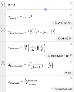
- Period of Orbit:
T= 2πr/v
Where r = a0n & v= c*alpha / n
- Energy Radiated per Period:
Using the Larmor formula,
EPer Period ∝ 1/n^5
- Total Energy Change Between Levels:
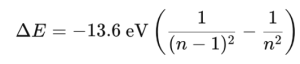
- Estimated Number of Revolutions:
Nrev ≃ delta E/ EPer Period
Ex: n=2, link to calculations
Lifetime:
The lifetime for one energy state to decay to its neighboring state could further be calculated by taking the product of Time per Period and number of revolutions, seen on that same Desmos script. This is another way that we can check our data to confirm that the model is accurate and appriproiitae. To corroborate our data and our calculations, the article “Semiclassical interpretation of spontaneous
transitions in the hydrogen atom” by Seidl provides a table with lifetimes of radiative decay of neighboring states. One method in the exact same way we did, sc(1B) and another, more robust integrated form sc(2B). We can compare our lifetime values with these values in Table 1 to again confirm the radiative model.
M Seidl and P O Lipas 1996 Eur. J. Phys. 17 25
With these checks, we can now research which model is best for this radiative process.
Abraham-Lorentz Self Force (Early 1900s):
After further research, we stumbled upon this force, with a derivation that stems directly from the Larmor formula, and seemingly rooted in fundamental physics. 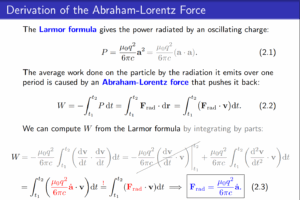
This self force was something that was difficult to implement into COMSOL because the ODE package that we were using was reliant on only 2nd order ODE’s. So after a lot of effort, we realized that we could just turn everything into state variables, break it down to 3 single order ODE (for the equation of motion for rx, meaning out system had in total 6 first order ODE’s) to allow the computer to calculate the third derivative of position.
After finally doing this, we saw that the solutions to the ODE’s were spirally outward or blowing up to infinity! Perplexed, we went to MatLab to try and confirm it wasn’t an issue with our numerical integrator, and sure enough it was not!
This led us to the literature, where we discovered that the strange spiraling outward behavior we observed was not a numerical artifact, but a known pathological feature of the self-force itself.
In particular, Marino (2003) provides a rigorous analysis of the nonrelativistic Lorentz–Dirac equation for an electron in a hydrogen-like atom. He proves that no matter what initial conditions are chosen, the electron will always eventually escape to infinity, either due to exponentially growing acceleration (runaway) or due to scattering with asymptotically vanishing acceleration. This completely contradicts naive expectations from classical electromagnetism, which suggest that the particle should spiral inward due to energy loss from radiation.
He states:
“We prove that for any choice of the initial data the particle always eventually escapes to infinity. Its acceleration either vanishes asymptotically, corresponding to a scattering process, or increases exponentially fast with time, with a so-called ‘runaway’ behaviour. No bound states of any type are possible.” (p. 11247)
The key insight is that even in an attractive Coulomb potential, the radiation reaction term dominates in such a way that instead of falling inwards, the particle accelerates away—a counterintuitive result that directly arises from the higher-order nature of the self-force equation. As Marino writes, this “appears as a remarkable contradiction to elementary physical intuition” (p. 11248)
M. Marino, J. Phys. A: Math. Gen. 36 (2003) 11247.
This is exactly what we saw, so although the Abraham-Lorentz Self Force seemed promising, this too will need to be sidelined.
Kowalski and the Gamma Parameter (1999):
To introduce energy loss into the hydrogen atom model, we turned to a paper that presents a classical framework for photon emission:
Marian Kowalski, Classical Description of Photon Emission from Atomic Hydrogen,
Physics Essays, Volume 12, Number 2, 1999.
Kowalski’s approach expresses radiation loss as a force term of the form: Frad=μγv
where μ is the reduced mass of the system, γ is an empirical parameter associated with radiation, and is the position vector. This term acts as a kind of “damping” that pulls the electron inward, simulating the radiation-induced loss of energy over time.
ODE for the x position, with corresponding ones in the y and z position.
mu * rxtt + (rx)/ rmag^3 + M2 * G1* rxt = 0
I added this force term directly to the ODEs governing the Coulomb interaction in the hydrogen atom model. Once implemented, the simulation produced behavior that aligned fairly well with Kowalski’s results.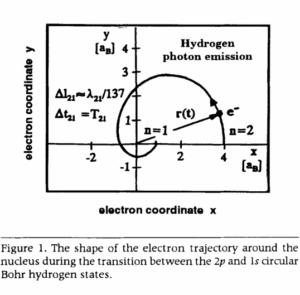
The model shows expected behavior: both energy and angular momentum decrease gradually over time. For example, when starting at n=2, the orbit transitions toward n=1, and the angular momentum (represented by ℓ) drops from 2 to 1, consistent with quantum predictions in a classical analog framework.
However, the decay isn’t a perfect match. The simulated trajectory tends to overshoot the final energy level slightly. We’re currently unsure whether this is due to differences in the radiation parameter γ, or if it stems from numerical inaccuracies in the integrator. To better control this, I implemented a stop condition in the solver that halts the simulation once a target energy is reached:
E_goal=−1/2 * 1/ ((n−1)^ 2), comp1.minop1(comp1.E) < E_Goal
This is what stops the computation in the video above, and as you see, the energy finally reaches the goal slightly past the (1,0) as excepted. That’s where the issue lies.
Wanting to see how this may apply to the Rydberg states ( n=100), we needed to figure out how he found the gamma parameters. he simply used ![]()
And rearranged for Gamma (pg. 323):
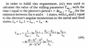 Using this equation, we could extrapolate this for those Rydberg states: You can view the math here
After finding this time constant, we saw that all the radiation happens in ONE ORBIT. This is not physically what happens. After looking further we see that Kowalski enforces this condition arbitrarily, and is something that is not physical.
Unfortunately, we will need to move off this radiative force.
Comparative Article: Hammond and Ford Models (2021):
G. Ares de Parga, S. Domínguez-Hernández, and E. Salinas-Hernández, Rev. Mex. Fis. 64 (2018) 187.
This article shows the Hammond and Ford models for a radiating hydrogen atom. This article takes these models and considers them both relativistically and non-relativistically, for our purposes we will look at the non-relativistically.
Ford (1991):
To understand the Ford equation, we can follow the notation found in Rajeev (S.G. Rajeev, Ann. Phys. 323 (2008) 2654.), which used the Landau-Lifshitz equation to get a 3rd order ODE that describes l^2. You can follow along in the paper, but the main idea is we can more easily represent the angular momentum with a ODE, then use that result to numerically solve for the I converted this to a MATLAB script.
MATLAB Script and Data
UPDAGTE!!!
Hammond (2008):
In the same way, we now model the system using the Hammond radiation reaction model. Following the formulation presented by Parga, I implemented the ordinary differential equation described in Equation (29) of the referenced paper. This equation of motion originates from Larmor radiation theory, which models energy loss due to electromagnetic radiation from an accelerating charge.
Structurally, the simulation shares many similarities with the Ford model: both use comparable initial conditions and rely on orbital dynamics around a central Coulomb potential. However, the ODE itself is different due to the nature of the radiation force. In this case, the force includes a damping term proportional to the velocity vector, scaled by 1 / r^4 v^2, as derived from the Hammond model.
Initial tests using ode45 or ode15s produced data with rotational counts in the range of ~10^4 (n=2), which was okay, however an unexpected behavior emerged: as the quantum number n increased, the number of rotations before decay decreased. Physically, this contradicts expectations. At larger n, the electron should begin at a greater radius, where radiation losses are smaller, and thus it should complete more revolutions before reaching the next energy level — not fewer. This inconsistency suggested a flaw in the numerical implementation.
To address this, I developed an alternative simulation method using a LeapFrog integrator.
Why the LeapFrog Method Works
The LeapFrog method is a second-order symplectic integrator, which is particularly well-suited for long-term simulations of conservative systems, such as orbital mechanics. Unlike MATLAB’s general-purpose solvers (ode45, ode15s), which are adaptive and prioritize error control, LeapFrog conserves geometric properties of the system like energy and phase-space structure over long time periods. This is crucial when dealing with very slow orbital decay, where integration errors can accumulate and distort the motion significantly.
Specifically, in the LeapFrog implementation:
- Velocities are updated by half a time step
- Positions are then updated by a full step
- Finally, velocities are updated again by another half step
This staggered update structure leads to excellent long-term stability, even in the presence of weak dissipative forces like those from radiation reaction.
With this method, I observed that the number of revolutions correctly increases with n, aligning with physical expectations. This confirms that the problem in the earlier implementation was not with the model itself, but with how the ODE was numerically solved. The LeapFrog method, although simpler and fixed-step, captured the cumulative effects of radiation loss more accurately in this specific context.
MATLAB Script and Data
Conclusion:
The Hammond model clearly provides the most accurate predictions, as the observed lifetimes and rotations align almost perfectly with the calculated values across all tested cases. Even at higher nn, the discrepancies remain negligible, demonstrating that the model reliably captures the underlying physics. The consistency between observed and theoretical results highlights its superiority over alternative approaches. Despite increasing computation times, the Hammond method’s precision makes it the best choice for modeling radiation reaction under a Coulomb field.