Ryan Yu | 8/12/25
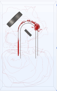
Ampere went to great lengths to suspend a magnet in the center of the rotating conductor structure. —— Figure 22 (h,s,m,r,p,q) were wooden fitters to suspend a magnet
In my modeling approach, I also keep a central stick magnet (Br of 1.3) in the domain, while changing the orientation of a second, larger magnet with a higher remanent flux density of 1.5.
Magnets used: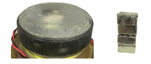
The cylindrical magnet was on the back of a loudspeaker! The one on the right is a stack of four K&J Magnets.
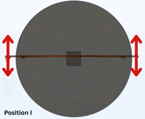
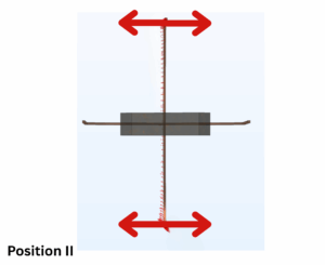
I tested five possible magnet configurations. In each, the stick magnet and the circular magnet are attracted to each other. You’ll notice that in the physical experiment, both magnets are beneath the device. I sought the orientation that would maximize the rotational velocity while keeping a magnet in the center, as this would bear the most resemblance to Ampere’s device.
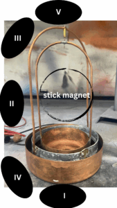
Preview:


I II III IV V
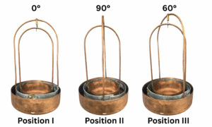
Running time-dependent studies is a difficulty in COMSOL. I had discovered this earlier when each computation and animation required hours to resolve, but in that case, I was simply testing if the device worked, and could run a courser mesh. In this study, I couldn’t use a coarser mesh as I needed accurate measurements. So instead, I took three positions in the rotation and ran a separate simulation for each:

 0°, 90°, 60°
–
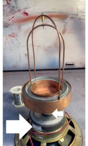
In each of the 12 simulations, I induced a current of .52541 A up the copper arms attached to the zinc, and down the copper arms to the inner cylinder. I then run an integration to gather the x,y, and z components of the lorentz force on each of the arms (as they are on opposite sides of the pivot point, they may oppose each other’s motion so I calculate torque separately to find the net torque myself). Additionally, I run point evaluations of the lorentz force in (N/m^3) as redundancy.
Legend for the data: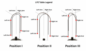
*Raw data of the Lorentz Force Evaluations are recorded in this spreadsheet. I’ll be referring to it in the next section.
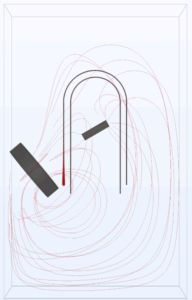
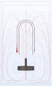
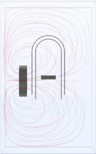
*Visuals of the Lorentz Force arrow plot from multiple angles (and my commentary) are recorded in this document
—
The first step to analyzing the data is determining which where, in each orientation, a lorentz force can generate torque. This is the direction we care about.
y-plane x-plane see below
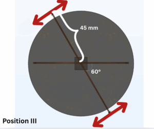
This, and the knowledge of the distance from the point of rotation to the leg (45 mm), allows us to calculate torque.

r=.045 m
*F is really Perpendicular Force; the force in the direction we care about.
First, we manually calculate the net Lorentz force for each of the 12 configurations from the Lorentz force evaluations. This is doneby taking the relevant component of Lorentz force for each arm and combining them. If they are of the same sign, they counteract each other and I subtract the absolute values. If they are different, I add the absolute values.
The first eight net forces in the x & y direction, respectively, for the 0° and 90° positions:
| (1,1) | −2.40×10⁻⁴ N |
| (1,2) | −5.26×10⁻³ N |
| (1,3) | 8.12×10⁻³ N |
| (1,4) | −2.95×10⁻³ N |
| (2,1) | −1.07×10⁻⁴ N |
| (2,2) | 9.00×10⁻⁴ N |
| (2,3) | −3.17×10⁻⁴ N |
| (2,4) | 4.23×10⁻⁴ N |
For Position 3 (60° orientation), the relevant component can be calculated according to sin(60)*Fx+cos(60)*Fy.
.5*Fx+.866*Fy
| (3,1) | -0.0001458502 left arm; 0.0000684936 right arm; =0.0002143438=2.14×10⁻⁴ N |
| (3,2) | -0.000211556 left arm; -0.000224678 right arm; =-0.000013122=-1.3×10⁻⁵ N |
| (3,3) | -0.000347744 left arm; 0.00022006 right arm; =0.000567804=5.68×10⁻⁴ N |
| (3,4) | -0.000814946 left arm; -0.000155028 right arm;=-0.000659918=6.60×10⁻⁴ N |
As the last step, we multiply each force by the distance from the point of rotation. Here we make a simplification and assume that the force acts from the straight portion of each arm, which is furthest from the point of rotation at 45 mm (which is also the radius of the zinc ring it is attached to) . Multiplying each value by .045, I find the following torques (in Nm):
| (1,1) | -1.08×10⁻⁵ |
| (1,2) | -2.367×10⁻⁴ |
| (1,3) | 3.654×10⁻⁴ |
| (1,4) | -1.3275×10⁻⁴ |
| (2,1) | -4.815×10⁻⁶ |
| (2,2) | 4.05×10⁻⁵ |
| (2,3) | -1.4265×10⁻⁵ |
| (2,4) | 1.9035×10⁻⁵ |
| (3,1) | 9.63×10⁻⁶ |
| (3,2) | -5.85×10⁻⁷ |
| (3,3) | 2.556×10⁻⁵ |
| (3,4) | 2.97×10⁻⁵ |
From this table, we can determine the optimal moments to switch magnet orientation in the physical experiment to maximize rotational velocity at each of the three positions. For counter-clockwise rotation, the greatest torque is achieved by running the experiment with (1,2), (2,3), (3,2). For clockwise rotation, it is (1,3), (2,2), (3,3).


