
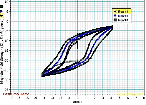
2. The frequency of an undamped oscillatory discharge affects the coercivity of the needle. The effect of this on a damped oscillatory discharge is yet to be determined.
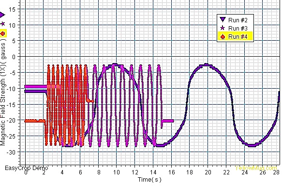
Below is the graph of undamped oscillatory discharges at different frequencies. It is easy to see that the higher the frequency of oscillation, the higher the coercivity of the material with slight changes in the remanance as well.
The reason for this is due to dissipating energy in the wires due to eddy currents, and this is best explained by Giorgio Bertotti in his book Hysteresis in Magnetism For Physicists, Materials Scientists, and Engineers:
“1.3.1 Eddy currents and magnetic losses
A particularly important example of dissipation mechanism giving rise to rate-dependent effects is represented by eddy currents in metallic systems. Let us consider the hysteresis loops of Fig. 1.11. These loops were measured on the same specimen of Si-Fe alloy for different frequencies f of oscillation of the applied field. The most evident feature is the substantial increase of the loop area and the change in the loop shape with increasing magnetization frequency. The loop area has an important physical meaning, because it represents the amount of energy irreversibly transformed into heat during one magnetization cycle. This derives from the fact, discussed in Chapter 12, that HdB represents the infinitesimal energy per unit volume injected in a magnetic specimen in the course of the magnetization process. The integral
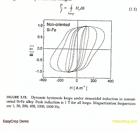
will thus represent the amount of work per unit volume performed by external sources and irreversibly transferred as heat to the thermal bath in one magnetization cycle. The quantity P is known as power loss, and P/f as loss per cycle.
When eddy current represent the dominant dissipation mechanism, one concludes that, if one knew the space-time distribution of the eddy current density j(r, t) inside the body, then one could immediately calculate the loss as
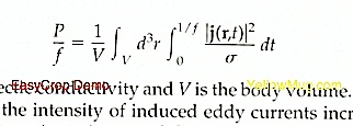
where sigma is the electric conductivity and V is the body volume. With increasing frequencies, the intensity of induced eddy currents increases accordingly, and this gives rise to increased dissipation and to larger loop areas, as observed in Fig. 1.11. How this qualitative statement can be made quantitative is an interesting physical problem in itself, and has important practical consequences in many applications. The eddy-current density j(r,t) is in general as complicated as magnetic domain structures are. Carrying out the space-time average involved in Eq. (1.2) requires a detailed analysis of magnetization processes, discussed in Chapter 12. However, some general conclusions can be summarized without going into quantitative details.
The first point to consider is that rate-dependent hysteresis introduces additional complications in the description of hysteresis loops. To identify a dynamic hysteresis loop, it is no longer sufficient to specify the peak value of the magnetization, as was the case for minor loops of Fig. 1.9. The magnetization frequency must also be known, as made clear by Fig. 1.11. But this is not enough. The particular waveform followed by the magnetization rate also has a role. Given the same magnetization frequency and peak magnetization, the dynamic loop traversed under sinusoidal magnetization will be in general different from the loop traversed under triangular magnetization, and so on. In the characterization of magnetic materials, the magnetic frequency f and the peak magnetization I(max) are always specified, and a sinusoidal magnetization rate is commonly required. An example of how the loss per cycle changes with frequency under these conditions is shown in Fig. 1.12. One often finds that the loss behavior is not far from the law
where the coefficients C0, C1, C2 may be functions of the peak magnetization I(max).
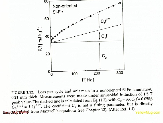
It is remarkable that laws of the type of Eq. (1.3) can exist at all. In fact, the loss, being the area of the hysteresis loop, might be expected to depend on a lot of details of the magnetization processes taking place along the loop. However, most of these details eventually turn out to be irrelevant, and only a few dominant features, described by the loss law, survive. This is even more remarkable when one considers that Eq. (1.3) applies to a broad class of different magnetic materials, characterized by largely different domain structures. An aspect of this generality is represented by loss separation. With this, one indicates the fact that it is possible to decompose the total loss at give frequency and peak magnetization into the sum of three contributions, known as hysteresis loss, classical loss, and excess loss. Loss separation is reflected by the structure of Eq. (1.3) itself. As will be discussed in Chapter 12, the presence of three terms is the result of the existence of three scales in the magnetization process. The scale associated with the hysteresis loss (the term C0 of Eq (1.3)) is the scale of the Barkhausen effect, where small domain wall segments make localized jumps between local minima of the system free energy, giving rise to localized eddy currents around the jumping walls. The second contribution is the so-called classcial loss (C1 in Eq. (1.3)). The scale associated with this term is the scale fixed by the specimen geometry. The classical loss is the loss calculated from Maxwell’s equations for a perfectly homogenous material with no domain structure. In this case, the boundary conditions of the problem, i.e., the specimen geometry, determine the result. Finally, the scale associated with the excess loss (C2 * sqrt(f) in Eq (1.3)) is the scale of magnetic domains. The excess loss arises from the eddy currents surrounding the active domain walls in motion under the driving action of the external field.
The three scales just mentioned are active at the same time, and it is by no means obvious why the existence of these scales should result in the fact that the space-time average of Eq (1.2) decomposes into the sum of three distinct terms. Actually, the fact that this turns out to be indeed the case is the main reason why it is possible to work out general laws for the loss description.”