Modern Recreation of Felix Savary’s Experiments Using Modern Technology

The damped oscillation equation is:

Using Simulink and Matlab, I set zeta to 1.8 and omega to 6. The only variable that I will change is the amplitude of the voltage generated by the power supply.  In Savary’s experiment, he had many needles at several distances from the wire. By changing the amplitude of the voltage generated by the power supply, we are simulating these differing distances from the wire.

Here is an example of the voltage outputted to the power supply (the amplitude is set to 6 volts):

Using DataStudio to capture the data of the PASCO magnetic field sensor, I made a graph which plotted the magnetic field strength (gauss) vs time:

There are two blips on the graph since I ran the simulation twice. The first time was run with an amplitude of +6 and the second time with an amplitude of -6. This way, we can estimate where the zero is on this graph so that we can record consistent data.

The second graph that I created plotted the magnetic field strength (gauss) vs. volts using an undamped oscillation simulation:

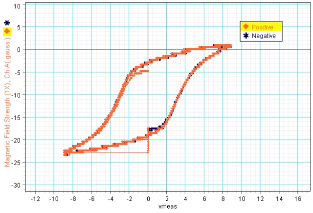
This graph is known as a hysteresis curve, or B-H graph. Click here for more information on what these curves mean. Notice that the graph is not centered at (0, 0). This just means that the magnetic field sensor was not zeroed while the needle was completely demagnetized, but this did not affect our results.

Click on the links below for the data captured while the voltage is set at different amplitudes. This simulates Felix Savary’s experiment of the polarizations of needles placed at different distances from a wire, as mentioned before.

Feel free to send an email if interested in complete data with accompanying graphs.